Müller Brown II

Previously on Müller Brown I

import numpy as np
from taps.paths import Paths
from taps.model import MullerBrown
from taps.coords import Coords
from taps.visualize import view

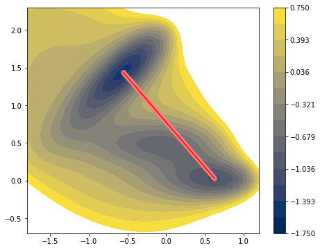
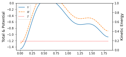
N = 300

x = np.linspace(-0.55822365, 0.6234994, N)
y = np.linspace(1.44172582, 0.02803776, N)

coords = Coords(coords=np.array([x, y]))
model = MullerBrown()
paths = Paths(coords=coords, model=model)
view(paths, viewer='MullerBrown')

<taps.visualize.view at 0x2b1e47592c90>

Müller Brown II

Here, we introduce a less fun but more practical tools in TAPS, Projector. Optimizing a pathway of an atomic system requires vast amount of computational time on the configuration space searching which in many case unfeasible. Projector class manipulates the coordinates system into smaller (usually) dimension so that user can reduce the configuration space for searching. For example, user can use the Mask projector that effectively hide some atoms from the PathFinder object so that position of some atoms can be fixed while optimizing the pathway. Surface reaction may use it useful restriction for a slab. Or user can optimize only the sine components of the pathway so user can effectively reduce the space to search. Or one may want to do it both. In the Projector class, there are three keywords domain, codomain, and pipeline. Unfortunately, domain and codomain keywords are exists as future usage. They are intended to controls the class of the pathway while prjoection into one to the other but currently it only exists as a concept. The third keyword, pipeline binds the multiple Projector class into one so that user can use multiple projector like one. For example, user can put Sine projector into the Masks pipeline so that some atoms are ignored and being fourie transformed. For simplicity, we are going to demonstrate only the Sine projector here.

Unfortunately, using Sine projector is not an automatic procedure. User has to put 4 additional kewords, total length of the coords, \(N\), a number of sine components \(N_k\), image of initial step init, and final reactant fin. Sine projector uses scipy.fftpack to conduct fast fourier transform. Sine use type 1 sine transformation, where

\[y_k = 2 \sum_{n=0}^{N-1} x_n \sin\left(\frac{\pi(k+1)(n+1)}{N+1}\right)\]

We have to fix the both end to 0. That gives us stability when removing high frequency components. Since it assumes the both end as 0, coordinate at both end should be given explcitley. Thus, user should manually specify the coordinate. Script below shows creation of the Sine projector and manipulate a sine components of that coordinate and visualize how it effected.

from taps.projectors import Sine
# We are going to use only the 30% of the coordinate information
Nk = N - 210
prj = Sine(N=N, Nk=Nk, init=paths.coords[:, 0].copy(), fin=paths.coords[:, -1].copy())
sine_coords = prj.x(paths.coords(index=np.s_[..., 1:-1]))

# Sine component manipulation
sine_coords[:, 1] = -5

new_coords = prj.x_inv(sine_coords)

paths.coords.coords[..., 1:-1] = new_coords.coords
view(paths, viewer='MullerBrown')

<taps.visualize.view at 0x2b1e464caf90>

Pathway optimization on the sine components.

Previouse MB example was conducted on the 2D Cartesian coordinate directly. In this example, we are going to use Sine projector during optimization process. Setting and kewords are same with previous example, with additional prj_search=True and prj=prj keyword inserted in DAO.

from taps.pathfinder import DAO

search_kwargs = {"method":"L-BFGS-B",
                  "options": {'disp': None,
                              'maxcor': 20,
                              'ftol': 2.220446049250313e-4,
                              'gtol': 1e-03,
                              'eps': 5e-6,
                              'maxfun': 1000,
                              'maxiter': 1000,
                              'iprint': -1, 'maxls': 100,
                              'finite_diff_rel_step': 1e-6}}

finder = DAO(Et=-0.45, muE=1., tol=1e-2, gam=1.,
             action_name = ['Onsager Machlup', "Energy conservation"],
             prj_search=True, sin_search=False,
             search_kwargs=search_kwargs,
             prj=prj)

paths.finder = finder
paths.coords.epoch=6
paths.search()

Action name  : Onsager Machlup + Energy conservation
Target energy: -0.45
Target type  : manual
muE          : 1.0
gamma        : 1.0
            Iter   nfev   njev        S   dS_max
converg :    149    156    156   2.2044   0.8695
converg :    151    161    161   2.2031   0.1778
jac_max > tol(0.01); Run without gradient
converg :    152    166    166   2.2029   0.0796

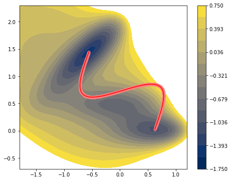
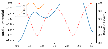
Below text is output of previous example, where cartesian coordinates were directly used as input \((N=300)\). But here we used only 30% \((Nk=90)\) of the coordinate information during optimization process. From that we get huge amount of gain in computatational cost but a little sacrifice of its accuracy without losing continuity required by action calculation.

Results in the previous example, Müller Brown I

Action name  : Onsager Machlup + Energy conservation
Target energy: -0.45
Target type  : manual
muE          : 1.0
gamma        : 1.0
            Iter   nfev   njev        S   dS_max
converg :   1011   1069   1069   2.1970   0.9060
converg :   1013   1075   1075   2.1955   0.4221
jac_max > tol(0.05); Run without gradient
converg :   1014   1080   1080   2.1951   0.4931

view(paths, viewer="MullerBrown")

<taps.visualize.view at 0x2b1fa93dd250>

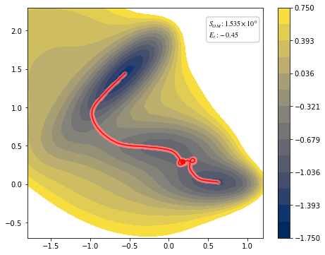
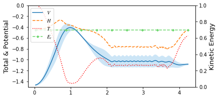
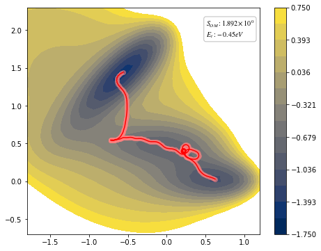
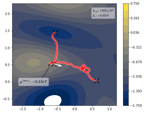
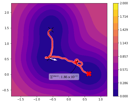
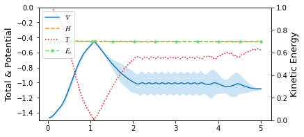
You can see through profile of the trajectory that it has lack of high frequency components.

Database construction

To utilize the data while we calculate the pathways, construction of proper database is postulated. ImageData class can save the calculation results of atomic or model system using below.

from taps.db.data import ImageData
imgdata = ImageData()
imgdata.add_data(paths, coords=(DxN or 3xDxN)size array)

TAPS aims for string method pathway calculation more effcient manner. meaning we insert some muller. In order to use I had to made the data abse

from taps.db.data import ImageData
imgdata = ImageData("mullerbrown.db")
#1. Projector
#2. Database
#3. Gaussian Potential

imgdata.add_data(paths, coords=paths.coords[..., [0, -1]])

{'image': [1, 3]}

imgdata.read_all()["image"][0], imgdata.read_all()["image"][1]

((array([-0.55822365,  1.44172582]),
  None,
  'Finished',
  1629604528.2957678,
  -1.4669951720995384,
  None,
  array([ 5.43788282e-08, -2.06867418e-07]),
  1629604528.2986429,
  None,
  None),
 (array([-0.3606111 ,  1.20532313]),
  None,
  'Finished',
  1629604528.298669,
  -0.3258472472753671,
  None,
  array([ 2.962832  , -2.67409004]),
  1629604528.3011174,
  None,
  None))

Gaussian Potential

With the data we constructed in this example, we are going to use it to construct Gaussian PES. Using only the 3 point of data, init, fin and middle point of the trajectory, We conconstruct the Gaussian Potential.

Kernel we are going to use here is standard (square exponential) kernel. Kernel looks like,

\[K(x_1, x_2) = \sigma_f e^{(x_1-x_2)^2/2l^2}\]

with zero mean, expectation value and covariance of the potential is

\[\mu = K_* (K_y+\sigma_n)^{-1} \mathbf{Y}\]

\[\Sigma = K_{**} + K_* K_y^{-1} K_*^{-1}\]

In the process of regression, where minimize the log likelihood, we

from taps.ml.gaussian import Gaussian
hyperparameters = {'sigma_f': 1, 'sigma_n^f': 1e-8, 'sigma_n^e':1e-6,
                   'l^2': 0.1}
hyperparameters_bounds = {'sigma_f': (1, 1), 'sigma_n^f': (1e-8, 1e-6), 'sigma_n^e':(1e-6, 1e-4), 'l^2': (1e-4, 4)}

#paths.finder.Et = -1.

paths.imgdata = imgdata
model = Gaussian(real_model=model,
                 hyperparameters=hyperparameters,
                 hyperparameters_bounds=hyperparameters_bounds)
paths.model = model
paths.add_data(index=[0, paths.N//3, -1])

{'image': [1, 10, 3]}

view(paths, viewer="MullerBrown", gaussian=True)

<taps.visualize.view at 0x2b1fa960ba90>

#paths.add_data(index=[0, -1])
paths.search()
view(paths, viewer="MullerBrown", gaussian=True)

Action name  : Onsager Machlup + Energy conservation
Target energy: -0.45
Target type  : manual
muE          : 1.0
gamma        : 1.0
            Iter   nfev   njev        S   dS_max
converg :    414    436    436   2.2993   0.1744
converg :    415    440    440   2.2991   0.2780
jac_max > tol(0.01); Run without gradient
converg :    416    444    444   2.2989   0.1004

<taps.visualize.view at 0x2b1fa91e8450>

Pathway optimization perfomed

We will going to use direct action optimization. There is some trivial case around it.