Müller Brown II

Previously on Müller Brown I

import numpy as np
from taps.paths import Paths
from taps.models import MullerBrown
from taps.coords import Cartesian
from taps.visualize import view

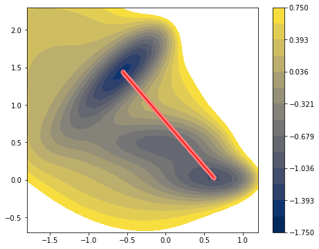
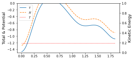
N = 300

x = np.linspace(-0.55822365, 0.6234994, N)
y = np.linspace(1.44172582, 0.02803776, N)

coords = Cartesian(coords=np.array([x, y]))
model = MullerBrown()
paths = Paths(coords=coords, model=model)
view(paths, viewer='MullerBrown')

<taps.visualize.view at 0x2ad2446bb750>

Müller Brown II

Here, we introduce a less fun but more practical tools in TAPS, Projector. Optimizing a pathway of an atomic system requires vast amount of computational time on the configuration space searching which in many case unfeasible. Projector class manipulates the coordinates system into smaller (usually) dimension so that user can reduce the configuration space for searching. For example, user can use the Mask projector that effectively hide some atoms from the PathFinder object so that position of some atoms can be fixed while optimizing the pathway. Surface reaction may use it useful restriction for a slab. Or user can optimize only the sine components of the pathway so user can effectively reduce the space to search. Or one may want to do it both. In the Projector class, there are three keywords domain, codomain, and pipeline. Unfortunately, domain and codomain keywords are exists as future usage. They are intended to controls the class of the pathway while prjoection into one to the other but currently it only exists as a concept. The third keyword, pipeline binds the multiple Projector class into one so that user can use multiple projector like one. For example, user can put Sine projector into the Masks pipeline so that some atoms are ignored and being fourie transformed. For simplicity, we are going to demonstrate only the Sine projector here.

Unfortunately, using Sine projector is not an automatic procedure. User has to put 4 additional kewords, total length of the coords, \(N\), a number of sine components \(N_k\), image of initial step init, and final reactant fin. Sine projector uses scipy.fftpack to conduct fast fourier transform. Sine use type 1 sine transformation, where

\[y_k = 2 \sum_{n=0}^{N-1} x_n \sin\left(\frac{\pi(k+1)(n+1)}{N+1}\right)\]

We have to fix the both end to 0. That gives us stability when removing high frequency components. Since it assumes the both end as 0, coordinate at both end should be given explcitley. Thus, user should manually specify the coordinate. Script below shows creation of the Sine projector and manipulate a sine components of that coordinate and visualize how it effected.

from taps.projectors import Sine
# We are going to use only the 30% of the coordinate information
Nk = N - 270
prj = Sine(N=N, Nk=Nk,
           init=paths.coords.coords[..., 0].copy(),
           fin=paths.coords.coords[..., -1].copy())
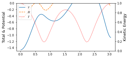
sine_coords = prj.x(paths.coords())

# Sine component manipulation
sine_coords.coords[:, 1] = -5

paths.coords = prj.x_inv(sine_coords)
view(paths, viewer='MullerBrown')

<taps.visualize.view at 0x2ad24ee15150>

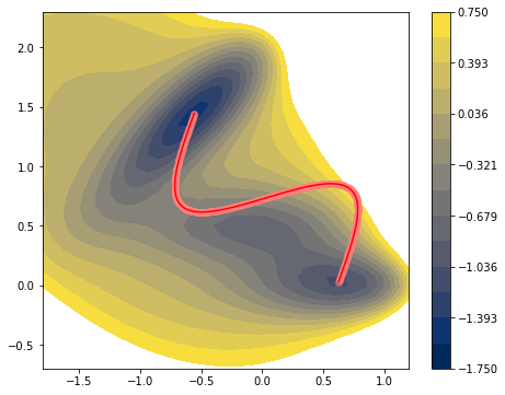
Pathway optimization on the sine components.

Previouse MB example was conducted on the 2D Cartesian coordinate directly. In this example, we are going to use Sine projector during optimization process. Setting and kewords are same with previous example, with additional prj_search=True and prj=prj keyword inserted in DAO.

from taps.pathfinder import DAO

action_kwargs = {
    'Onsager Machlup':{
        'gam': 1.,
    },
    'Energy Restraint':{
        'muE': 1.,
        'Et': -0.45
    }
}

search_kwargs = {"method":"L-BFGS-B"}

finder = DAO(action_kwargs=action_kwargs,
             search_kwargs=search_kwargs,
             prj=prj)

paths.finder = finder
paths.coords.epoch=6
paths.search()

=================================
      DAO Parameters
=================================
Onsager Machlup
  gam        : 1.0

Energy Restraint
  muE        : 1.0
  Et         : -0.45

            Iter   nfev   njev        S   dS_max
Converge :    496    535    535   2.0390   0.0002
Converge :    497    538    538   2.0390   0.0007

=================================
            Results
=================================
 Onsager Machlup             : 1.4683439570562704
 Energy Restraint            : 0.5706377155193327
 Total S                     : 2.038981672575603

Below text is output of previous example, where cartesian coordinates were directly used as input \((N=300)\). But here we used only 10% \((Nk=30)\) of the coordinate information during optimization process. From that we get huge amount of gain in computatational cost but a little sacrifice of its accuracy without losing continuity required by action calculation.

Results in the previous example, Müller Brown I

=================================
      Parameters
=================================
Onsager Machlup
  gam        : 1.0

Energy Restraint
  muE        : 1.0
  Et         : -0.45

            Iter   nfev   njev        S   dS_max
Converge :   9784  10021  10021   1.8258   0.0070
Converge :   9785  10040  10040   1.8258   0.0070

=================================
            Results
=================================
 Onsager Machlup             : 1.2556032942672488
 Energy Restraint            : 0.5702371630130022
 Total S                     : 1.825840457280251

view(paths, viewer="MullerBrown")

<taps.visualize.view at 0x2ad24f0b4bd0>

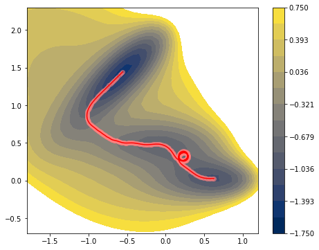
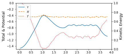
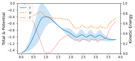
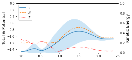
You can see through profile of the trajectory that it has lack of high frequency components.

Database construction

To utilize the data while we calculate the pathways, construction of proper database is postulated. ImageData class can save the calculation results of atomic or model system using below.

from taps.db import ImageData
imgdb = ImageData()
imgdb.add_image_data(paths, coords=(DxN or 3xDxN)size array)

TAPS aims for string method pathway calculation more effcient manner. meaning we insert some muller. In order to use I had to made the data abse

from taps.db import ImageDatabase
imgdb = ImageDatabase(filename="mullerbrown.db")
imgdb.add_image_data(paths, coords=paths.coords(index=[0, -1]))

[1, 2]

Gaussian Potential

With the data we constructed in this example, we are going to use it to construct Gaussian PES. Using only the 3 point of data, init, fin and middle point of the trajectory, We conconstruct the Gaussian Potential.

Kernel we are going to use here is standard (square exponential) kernel. Kernel looks like,

\[K(x_1, x_2) = \sigma_f e^{(x_1-x_2)^2/2l^2}\]

with zero mean, expectation value and covariance of the potential is

\[\mu = K_* (K_y+\sigma_n)^{-1} \mathbf{Y}\]

\[\Sigma = K_{**} + K_* K_y^{-1} K_*^{-1}\]

In the process of regression, where minimize the log likelihood.

from taps.models import Gaussian

paths.imgdb = imgdb

model = Gaussian(real_model=MullerBrown())
paths.model = model

paths.add_image_data(index=[0, paths.coords.N // 2, -1])

from scipy.optimize import minimize, Bounds
from taps.models.gaussian import Likelihood
loss_fn = Likelihood(kernel=model.kernel, mean=model.mean,
                     database=imgdb, kernel_prj=model.prj)
x0 = model.kernel.get_hyperparameters()
res = minimize(loss_fn, x0, method='L-BFGS-B', bounds=Bounds([1e-5, 1e-4, 0., 0.], [np.inf, 1e2, 1e-4, 1e-6]))

model.set_lambda(imgdb, hyperparameters=res.x)

#paths.model.kernel.hyperparameters['sigma_f'] = 0.5
#paths.model.kernel.hyperparameters['l^2'] = 0.1
view(paths, viewer="MullerBrown", gaussian=True)

<taps.visualize.view at 0x2ad250824550>

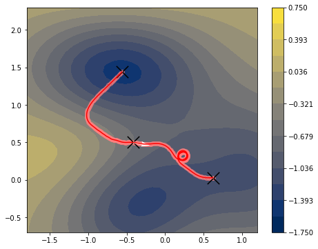
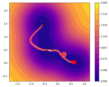
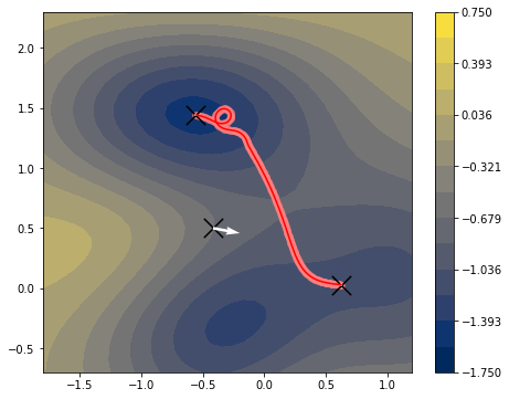
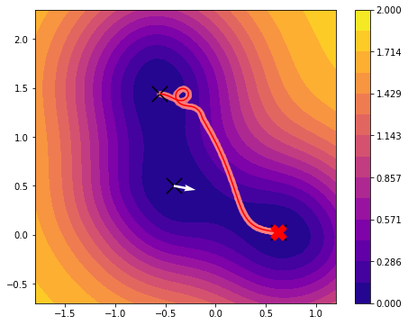
\(\mu\) and \(\Sigma\) Maps

You can see the second and third map images that depicting mean expectation value, \(\mu\), and uncertainty map, \(\Sigma\) with additional information plotted on the map such as maximum uncertainty or maximum estimated potential.

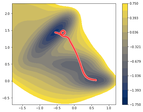
It looks totally different from real PES, the first map. We will shows you how we approximate the PES near the minimum energy pathway (MEP) to real one. We will finish this tutorial by optimizing the pathway based on the Gaussian PES.

paths.finder.action_kwargs['Energy Restraint'].update({'Et': -1.2})
paths.search()
view(paths, viewer="MullerBrown", gaussian=True)

=================================
      DAO Parameters
=================================
Onsager Machlup
  gam        : 1.0

Energy Restraint
  muE        : 1.0
  Et         : -1.2

            Iter   nfev   njev        S   dS_max
Converge :    735    783    783  17.7268   0.0002
Converge :    736    786    786  17.7268   0.0013
sigma_f    : 3.2920229051552785
l^2        : 0.6133555048172792
sigma_n^e  : 0.0001
sigma_n^f  : 9.8974327002846e-07
=================================
            Results
=================================
 Onsager Machlup             : 0.7293807792450809
 Energy Restraint            : 16.997400946464047
 Total S                     : 17.726781725709127

<taps.visualize.view at 0x2ad250940a90>

Machine Learning potential

prerequisites: pytorch